Inertial Easing
22/03/2026
A little while ago a Japanese programmer and visual artist Baku posted on twitter about a technique (that I presume he invented) called Inertial Easing. It resembled the kind of spring smoothing techniques I've been interested in for a long time. The main difference for this technique appeared to be that it used easing functions, which are common in game development, and a lot of people will already be familiar with.
I noted down the name "Inertial Easing" as something to look up in the future, but recently when I searched for it again I couldn't find any trace of it on the web other than this Open Processing Demo. That made me think it was probably time to try and reverse engineer whatever I could and see if I could preserve it somewhat.
There were some elements of Baku's original mathematics I didn't quite understand, or didn't quite make sense to me - but in the end I think I have something that contains all of the core ideas and seems to produce similar enough results.
So let me try to explain my interpretation of Inertial Easing:
Inertial Easing starts with the following problem statement (which might sound familiar to those who have read my article on springs). If we have a value, changing with a given velocity, and a target value we want to interpolate towards within some fixed time, how do we find a smooth path that brings us there:
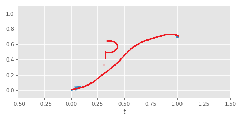
One way to find this smooth path is to fit some simple function such as a cubic function to the initial velocity and target to find a curve that reaches the goal at the given time:
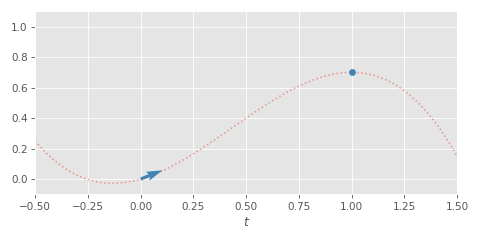
Once we've fitted the function, we can evaluate it over time to smoothly transition towards our target - re-fitting the function, and resetting the time, whenever the target changes.
The problem we have is that whenever our target changes our time "resets", meaning that if the target is jumping around frequently we're always exponentially approaching it, rather than reaching it in a fixed time:
What would be nice is if, as well as fitting a curve that takes us toward a target, we could also choose some kind of initial starting time \( t \) along the curve, such that if we were already close to the target we'd start further along this curve, and the blend would not take as long - we'd reach it without having to reset our time back to zero.
Well, this is basically the core idea behind Inertial Easing!
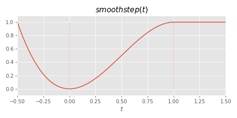
This time, the function we're going to fit will be an easing function such as smoothstep, with negative part included (this is important as it allows us to change direction when the initial velocity is facing away from the target):
In code:
// Scaled smoothstep including negative section
float smoothstep(float t, float s)
{
    return s * (t > 1.0f ? 1.0f : 3*t*t - 2*t*t*t);
}
We also are going to make use the derivative with respect to time:
// Scaled smoothstep derivative including negative section
float smoothstep_dt(float t, float s)
{
    return s * (t > 1.0f ? 0.0f : 6*t - 6*t*t);
}
In this case I've set it up so that we have two parameters to the function: a time value t, and a scale value s, which we can use to scale the vertical axis of the function:
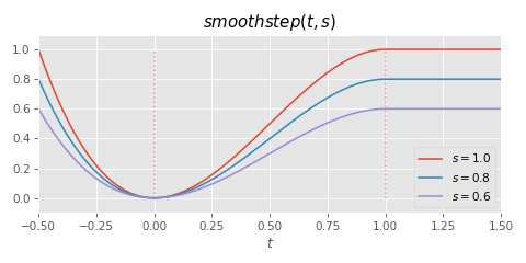
If we can fit these parameters correctly each time the target changes, then we just need to play-out the rest of this function by accumulating the time value t like we did with our cubic fit.
// Check if target changed
if (IsMouseButtonDown(MOUSE_RIGHT_BUTTON))
{
    if (g != GetMousePosition().y)
    {
        // Update Target
        g = GetMousePosition().y;

        // Solve for smoothstep parameters `s` and `t`
        smoothstep_solve(et, es, g - x, smoothstep_dt(et, es));

        // Set the offset to the difference between the target and current eased value
        eo = x - smoothstep(et, es);
    }
}

// Update the easing time
et += dt / max(blendtime, 1e-4f);

// Update the eased value
x = eo + smoothstep(et, es);

// Update Time
t += dt;
And this time, since we also fit the time value t, we're not going to be constantly lagging behind if the target keeps changing.
The question now becomes how to implement smoothstep_solve - how do we actually find appropriate values for t and s when the target changes.
The way to think about it is in terms of constraints. First, we want the velocity to be continuous when we transition - that is - even if our t and s parameters change, the velocity of the the newly fitted easing function should match what we had before we re-fit the parameters. Second, we want the final position of the easing function (i.e. when \( t = 1 \) ) for it to have reached our target value.
While Baku formulates this in a generic way, the code is a lot more simple if we choose a concrete easing function. In this case I'm going to show the derivation for the \( smoothstep \) easing function from before.
First, we can make the observation that as we change the scale parameter \( s \) of our easing function, the velocity \( v \) of the easing function changes directly proportionally. This means if we have some velocity we want the easing function to have for some given time \( t \), we can ensure this is the case by picking the appropriate value for \( s \). In this case it can be computed by dividing the velocity \( v \) by the un-scaled velocity of the easing function at time \( t \) will give us the correct scaling factor:
\begin{align*} s &= \frac{v}{ \tfrac{d}{dt} smoothstep(t, 1)} \end{align*}
So the scaling factor \( s \), initial velocity \( v \), and time \( t \) are all linked by the above equation. That means if we are provided an initial velocity \( v \), and can find a time \( t \) - our scaling factor \( s \) is automatically implied by the above.
The question now becomes how to find the time value \( t \). For this we make use of our second constraint: we need to pick a time which results in us ending up at the given target \( x \) once the full function has elapsed.
The difference between final location of the \( smoothstep \) function and initial location for scale \( s \) and time \( t \) will be: \( smoothstep(1, s) - smoothstep(t, s) = s - smoothstep(t, s) \). This we need to set equal to our target location \( x \) and solve for \( t \):
\begin{align*} x &= s - smoothstep(t, s) \end{align*}
We can start by expanding the \( smoothstep \) function:
\begin{align*} x &= s - s \cdot (3 \cdot t^2 - 2 \cdot t^3) \end{align*}
And then we can factor out the \( s \):
\begin{align*} x = s \cdot (1 - (3 \cdot t^2 - 2 \cdot t^3)) \end{align*}
We can replace \( s \) in the above with our function that links the scale to the velocity:
\begin{align*} x &= \frac{v}{ \tfrac{d}{dt} smoothstep(t, 1)} \cdot (1 - (3 \cdot t^2 - 2 \cdot t^3)) \end{align*}
Which we can expand out again.
\begin{align*} x = \frac{v}{6 \cdot t - 6 \cdot t^2} \cdot (1 - (3 \cdot t^2 - 2 \cdot t^3)) \end{align*}
This we can solve for \( t \) as follows. First we re-arrange to get a quadratic.
\begin{align*} x &= \frac{v}{6 \cdot t - 6 \cdot t^2} \cdot (1 - (3 \cdot t^2 - 2 \cdot t^3)) \\ \tfrac{x}{v} &= \frac{1 - (3 \cdot t^2 - 2 \cdot t^3)}{6 \cdot t - 6 \cdot t^2} \\ \tfrac{x}{v} &= \frac{(t - 1)^2 \cdot (2 \cdot t + 1)}{-6 \cdot t \cdot (t - 1)} \\ \tfrac{x}{v} &= \frac{(t - 1) \cdot (2 \cdot t + 1)}{-6 \cdot t} \\ \tfrac{x}{v} &= \frac{2 \cdot t^2 - t - 1}{-6 \cdot t} \\ \tfrac{x}{v} &= -\tfrac{2 \cdot t}{6} + \tfrac{1}{6} + \tfrac{1}{6 \cdot t} \\ \tfrac{6 \cdot x}{v} &= -2 \cdot t + 1 + \tfrac{1}{t} \\ 0 &= -2 \cdot t + 1 + \tfrac{1}{t} - \tfrac{6 \cdot x}{v} \\ 0 &= 2 \cdot t - 1 - \tfrac{1}{t} + \tfrac{6 \cdot x}{v} \\ 0 &= \frac{-t \cdot v - v + 2 \cdot v \cdot t^2 + 6 \cdot t \cdot x}{t \cdot v} \\ t \cdot v \cdot 0 &= -t \cdot v - v + 2 \cdot v \cdot t^2 + 6 \cdot t \cdot x \\ 0 &= 2 \cdot v \cdot t^2 + (6 \cdot x - v) \cdot t - v \\ \end{align*}
Which we can then solve with the quadratic formula.
\begin{align*} t &= \frac{-b \pm \sqrt{b^2 - 4 \cdot a \cdot c}}{2 \cdot a} \\ a &= 2 \cdot v \\ b &= 6 \cdot x - v \\ c &= -v \\ \end{align*}
Which gives...
\begin{align*} t_0 &= \frac{v - 6 \cdot x + \sqrt{(6 \cdot x - v)^2 + 8 \cdot v^2}}{4 \cdot v} \\ t_1 &= \frac{v - 6 \cdot x - \sqrt{(6 \cdot x - v)^2 + 8 \cdot v^2}}{4 \cdot v} \\ \end{align*}
(Aside: for those that feel a bit intimidated by these long mathematical derivations in my blog - perhaps it is reassuring to know that I almost always solve these backwards. That is - I ask Wolfram Alpha or some other tool for the solution, and then I try to go backwards from the solution to my original equation. That works best for me: I don't waste time searching for a solution that may or may not exist, it's often easier to solve when you know both end-points, and I still come away convinced it works and feeling like I understand all the individual steps involved.)
As we can see, there are two solutions. For the most simple implementation of Inertial Easing, we can just always take the first solution, which will always get us to the target in the quickest time.
There are some edge cases to deal with first though. If the initial velocity is close to zero then the best fitting time and scale values are ambiguous, so we simply start from zero and set the scale to make sure we get to the target. If the target is negative we simply invert it (along with the velocity) and solve again, then negate the solved for scale value. This ensures we're always dealing with a positive target value \( x \) for our quadratic solve. Putting it all together in code:
// Solve for smoothstep parameters `t` and `s` given new target `x` and velocity `v`
void smoothstep_solve(float& t, float& s, float x, float v, float eps=1e-8f)
{
    // If velocity is zero start from time zero with scale to match `x`
    if (fabsf(v) < 1e-8f)
    {
        t = 0.0f;
        s = x;
        return;
    }

    // If `x` is negative then invert signs and re-solve
    if (x < 0.0f)
    {
        smoothstep_solve(t, s, -x, -v);
        s = -s;
        return;
    }

    // Find the time that solves for the given `x` and `v`
    t = (v - 6*x + sqrtf(max((6*x - v)*(6*x - v) + 8*v*v, eps))) / (4*v);

    // Find the un-scaled velocity at the fitted time
    float vt = smoothstep_dt(t, 1.0f);

    // Find the scaling factor so that the velocity at the fitted time matches
    s = fabsf(vt) < eps ? 0.0f : v / vt;
}
Here is what it looks like:
This system has a number of nice properties.
First, just like a spring, we can smooth out sudden discontinuities. However, unlike a spring, we can also guarantee that the target will be reached exactly in less than \( 1.5 \times \) the blend time.
Second, with this easing function we get symmetric starts and stops - a real S-shape - which might be preferable to the lopsided critical spring function.
Finally, since we are using an easing function, in-between target changes we can easily estimate exactly how long it will take for us to reach the target, and could use this to compute things like the distance travelled if (for example) this was being used in part of a movement model for a character controller.
There is a final aspect which can be a pro or con depending on how you see it: we never overshoot when the target is in the same direction as the velocity. This is good if you want to avoid overshooting, since it gives you good knowledge of when overshooting is expected and when it isn't. The downside is that in some extreme cases when a new target is placed just in front of the current value you can get very large accelerations as the system comes to an immediate stop (you might have noticed this happen in the previous video):
There is something we can do about this - we can use the other solution to the quadratic. Most of the time this solution is not helpful - either being a time value \( >1 \), or some very large negative number matched with a very small scaling factor, that results in the system taking an eternity to reach the target.
However, at the point where the target crosses the current position this other solution approaches \( -0.5 \), and it can make sense to choose it instead, causing us to over-shoot the target and return back around, taking \( \sim 1.5 \times \) the blend time, rather than snapping instantly to it. We can configure exactly how much tolerance we want to give here - and at what point we prefer to overshoot and take a long blend over a short one.
// Solve for smoothstep parameters `t` and `s` given new target `x` and velocity `v`
void smoothstep_solve(
    float& t, float& s, float x, float v, float overshoot = 0.05f, float eps=1e-8f)
{
    // If velocity is zero start from time zero with scale to match `x`
    if (fabsf(v) < 1e-8f)
    {
        t = 0.0f;
        s = x;
        return;
    }

    // If `x` is negative then invert signs and re-solve
    if (x < 0.0)
    {
        smoothstep_solve(t, s, -x, -v);
        s = -s;
        return;
    }

    // Find the possible times that solve for the given `x` and `v`
    float t0 = (v - 6*x + sqrtf(max((6*x - v)*(6*x - v) + 8*v*v, eps))) / (4*v);
    float t1 = (v - 6*x - sqrtf(max((6*x - v)*(6*x - v) + 8*v*v, eps))) / (4*v);

    // Overshoot if the alternative time is between -0.5f and -(0.5f + overshoot)
    t = -0.5f > t1 && t1 > -(0.5f + overshoot) ? t1 : t0;

    // Find the un-scaled velocity at the fitted time
    float vt = smoothstep_dt(t, 1.0f);

    // Find the scaling factor so that the velocity at the fitted time matches
    s = fabsf(vt) < eps ? 0.0f : v / vt;
}
I've found a value of around 0.05 seems to work pretty well - and limits overshooting only to what would be the most visually jarring cases. Here is what it looks like:
So that pretty-much summarises my investigations into Inertial Easing. You can find all the source code for this article here. Overall it's a cool technique that could have a lot of nice applications. I can see it being used as a general purpose spring and/or inertialization/dead-blending alternative or as part of a movement model, or as a way of smoothing out path-finding - perhaps even as some kind of spline. It might give some odd results when applied to vectors since the time-of-arrival for each component will likely be different - so might be more effective applied to interpolation weights or something like that. Let me know if you find any interesting uses for this technique! As always, thanks for reading.