Fitting Code Driven Displacement

Created on Feb. 7, 2022, 8:28 a.m.

In my article code vs data driven displacement I talked about how the code driven displacement of a character (i.e. the movement as described by some simple system such as a critically damped spring) should ideally match the data driven displacement of the character - the movement as described by the the actual animation or motion capture data.

In that article I showed how we can do some basic data visualization such as comparing histograms to try and help us find parameters for the code driven displacement that match. In this article I'm going to show one idea for how we can automatically extract matching parameters for our code driven setup directly from our motion capture data.

Assuming we're using critically damped springs as the main component in our code driven displacement, then essentially we have three parameters we need to fit for each mode we might be interested in (such as running, walking, or strafing etc). These parameters are:

The max velocity
The velocity "half-life"
The facing angle "half-life"

The "max velocity" is a relatively straight forward parameter, which we can compute from motion capture data simply by finding the largest magnitude of the velocity the actor travels at.

The second two are where the trouble lie. Not only is there no obvious way to compute these from motion capture data, but they are not even particularly intuitive for animators or designers to set.

In reality the "half-life" controls a kind of fuzzy "reaction time" - given a new goal velocity or facing angle, the "half-life" dictates (approximately) how long (in seconds) it will take for the character to get half the way there.

We can see this approximate relationship if we plot some different half-lives, for a spring with a starting state of 0 and a goal of 1:

halflives

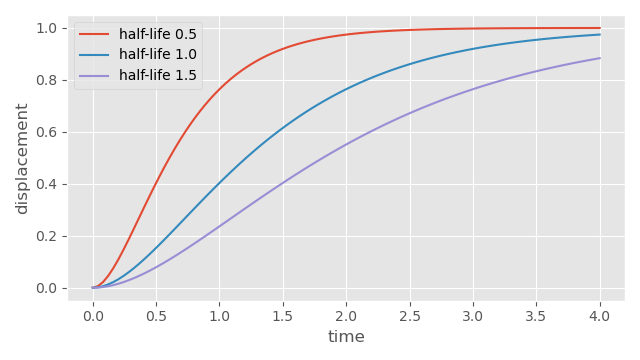
There are two simple but important observations we can make here: first, that if we scale the vertical axis (such as by picking a goal further away), the shape of the spring's movement will not actually change at all - the half-life based control means it will simply move a greater distance in the same amount of time to compensate. And second, that the smaller the half-life, the steeper the gradient achieved as the spring moves toward the goal more quickly.

The gradient here can be computed exactly using the derivative of our critical spring equation:

\begin{align*} x_{t} &= j_0 \cdot e^{-y \cdot t} + t \cdot j_1 \cdot e^{-y \cdot t} + c \\ v_{t} &= v_0 \cdot e^{-y \cdot t} - t \cdot j_1 \cdot y \cdot e^{-y \cdot t} \\ a_{t} &= t \cdot j_1 \cdot y^2 \cdot e^{-y \cdot t} - j_1 \cdot y \cdot e^{-y \cdot t} - v_0 \cdot y \cdot e^{-y \cdot t} \\ \end{align*}

where the variables here are the same as we used in the Spring Roll Call. In Python we might therefore write the critically damped spring function as follows...

def halflife_to_damping(halflife, eps=1e-5):
    return (4.0 * 0.69314718056) / (halflife + eps)

def damping_to_halflife(damping, eps=1e-5):
    return (4.0 * 0.69314718056) / (damping + eps)

def critical_spring_damper(
    x,        # Initial Position
    v,        # Initial Velocity
    x_goal,   # Goal Position
    halflife, # Halflife
    dt        # Time Delta
    ):
    
    y = halflife_to_damping(halflife) / 2.0
    j0 = x - x_goal
    j1 = v + j0*y
    eydt = np.exp(-y*dt)

    return (
        eydt*(j0 + j1*dt) + x_goal,   # Next Position
        eydt*(v - j1*y*dt),           # Next Velocity
        eydt*(y*j1*dt*y - y*j1 - y*v) # Next Acceleration
    )

And if we actually plot the gradient of these different springs, we can see visually what maximum velocity is achieved.

halflives grad

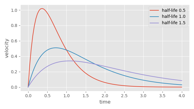
So for anything we are interested in smoothing with a spring (such as character velocity, or facing angle), the half-life also controls the maximum value we will observe for the derivative of this value (such as character acceleration, or angular velocity).

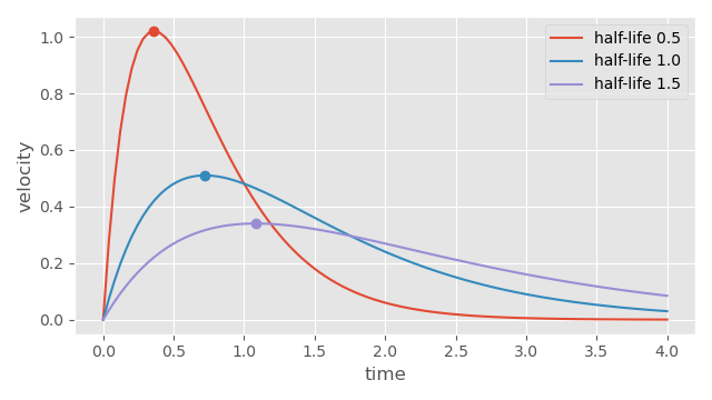
If we want to know the time at which this maximum occurs, we can find it by taking the second derivative of our spring equation, setting its negation to be equal to zero, and solving for time \( t \):

\begin{align*} a_{t} &= t \cdot j_1 \cdot y^2 \cdot e^{-y \cdot t} - j_1 \cdot y \cdot e^{-y \cdot t} - v_0 \cdot y \cdot e^{-y \cdot t} \\ 0 &= -(t_{max} \cdot j_1 \cdot y^2 \cdot e^{-y \cdot t_{max}} - j_1 \cdot y \cdot e^{-y \cdot t_{max}} - v_0 \cdot y \cdot e^{-y \cdot t_{max}}) \\ 0 &= -e^{-y \cdot t_{max}} \cdot ( t_{max} \cdot j_1 \cdot y^2 - j_1 \cdot y - v_0 \cdot y) \\ 0 &= -t_{max} \cdot j_1 \cdot y^2 + j_1 \cdot y + v_0 \cdot y \\ t_{max} \cdot j_1 \cdot y^2 &= j_1 \cdot y + v_0 \cdot y \\ t_{max} \cdot j_1 \cdot y &= j_1 + v_0 \\ t_{max} &= \frac{j_1 + v_0}{j_1 \cdot y} \\ \end{align*}

Notice how we make the \( e^{-y \cdot t_{max}} \) disappear by just solving for the right hand side of the multiplication to be equal to zero. We can write this solution in code as...

def spring_maximum_velocity_time(x, v, x_goal, halflife):
    y = halflife_to_damping(halflife) / 2.0
    j0 = x - x_goal
    j1 = v + j0*y
    return (j1 + v) / (j1 * y)

Then, by plugging this time back into our spring equation, we can get the actual velocity at this time.

halflives grad peaks

One use of this formula is to predict the maximum value of the derivative of the thing we are smoothing with the spring. For example, for a character changing velocity from \( 0\ m/s \) to \( 5\ m/s \) smoothed using a spring with a half-life of \( 0.2\ s \), we can compute that the character will have a maximum acceleration of \( 0.14\ m/s^2 \)

But, more importantly, by rearranging this equation we can go in the opposite direction - and compute the half-life that corresponds to a given maximum derivative value. In the general case this is pretty difficult to solve, but if we plug in initial conditions \( x_0 = 0 \), \( v_0 = 0 \), \( g = 1 \) such as in our simple ramp-up situation shown above the solution is simple.

First \( j_1 \) simplifies to \( -y \):

\begin{align*} j_1 &= v_0 + (x_0 - g) \cdot y \\ j_1 &= 0 + (0 - 1) \cdot y \\ j_1 &= -y \\ \end{align*}

Then \( t_{max} \) itself reduces down to simply \( \frac{1}{y} \):

\begin{align*} t_{max} &= \frac{j_1 + v_0}{j_1 \cdot y} \\ t_{max} &= \frac{-y + 0}{-y \cdot y} \\ t_{max} &= \frac{1}{y} \\ \end{align*}

Which greatly simplifies our spring velocity equation and allows us to solve for \( y \) (from which we will be able to compute the half-life):

\begin{align*} v_{t} &= v_0 \cdot e^{-y \cdot t} - t \cdot j_1 \cdot y \cdot e^{-y \cdot t} \\ v_{max} &= v_0 \cdot e^{-y \cdot t_{max}} - t_{max} \cdot j_1 \cdot y \cdot e^{-y \cdot t_{max}} \\ v_{max} &= 0 \cdot e^{-\tfrac{y}{y}} - \tfrac{1}{y} \cdot -y \cdot y \cdot e^{-\tfrac{y}{y}} \\ v_{max} &= y \cdot e^{-1} \\ y &= v_{max} \cdot e \\ \end{align*}

If we want to do the same computation with a larger goal value than 1, we can simply scale \( v_{max} \) since we observed that the overall shape of the spring does not change as the vertical axis scales:

def maximum_spring_velocity_to_halflife(x, x_goal, v_max):
    return damping_to_halflife(2.0 * ((v_max / (x_goal - x)) * np.e))

Then, for example, given a change in character velocity from \( 0\ m/s \) to \( 5\ m/s \), with an expected maximum character acceleration of \( 2\ m/s^2 \), we can compute that we need to use a spring with a half-life of \( 1.27\ s \).

Not only is this a much more intuitive control for animators and designers to tweak, but since it's a real-world measurable value, it also gives us the ability to potentially extract it from motion capture data.

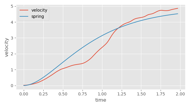
To test this idea out, I took a stand-to-run clip from the data used in code vs data driven displacement and plotted the velocity and acceleration profiles:

root_velocity

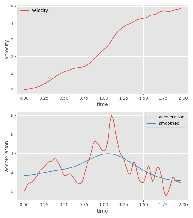
While we can compute directly here that the maximum velocity is around \( 4.86\ m/s \), if we had a large dataset we might want to compute something like the maximum velocity sustained over 0.5 seconds to be a bit more robust to outliers or other errors in the data instead.

The acceleration profile is more unstable, with a lot of movement up and down. If we smooth the signal and look at the maximum again, we can get a value of around \( 3.94\ m/s^2 \).

By plugging these two numbers into our previous equation we can see that a spring with a half-life of \( 0.63\ s\) should match this situation well. We can plot a spring with those properties on top to test exactly that:

root_velocity_spring

Not such a bad fit! We can also do the same for facing direction. Here I found a plant and turn clip, and plotted the facing angle over time, as well as the angular velocity over time:

root_angle

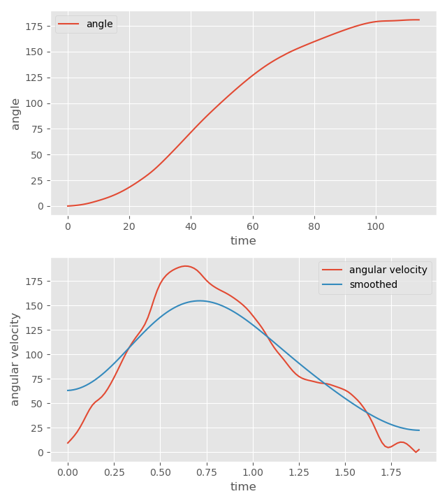
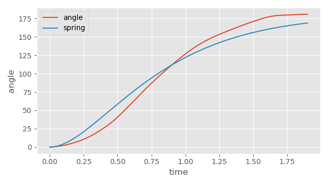
Here we can see that through a 180 degree turn, the character achieves a maximum (smoothed) angular velocity of \( 154.68\ ^{\circ}/s \). Plugging these numbers into our equation gives a corresponding half-life of \( 0.60\ s \). If we overlay the plots again we can see a fairly nice match:

root_angle_spring

Just for fun I found online a very approximate velocity and acceleration profile for Usain Bolt:

bolt_velocity

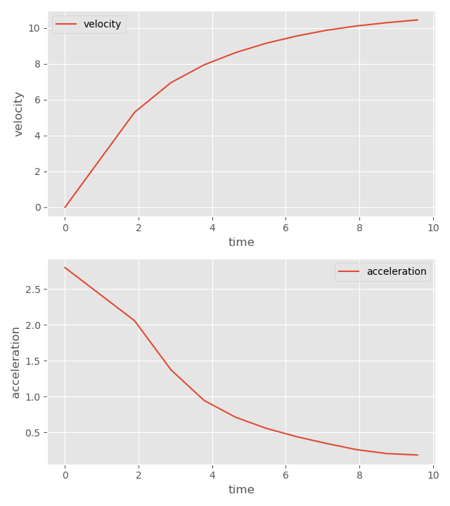
Here we can see Usain Bolt has a max velocity of roughly \( 10.44\ m/s \) and max acceleration of roughly \( 2.80\ m/s^2 \). We can compute that this corresponds to a half-life of \( 1.90 \). Like before, we can plot this on top to see how it looks:

bolt_velocity_spring

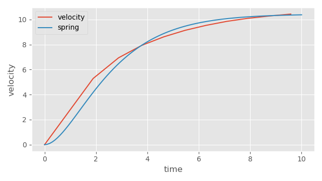
Again, a pretty good fit.

So next time you're in the pub with some sports-fans and want to impress them with a surprising and rare sports stat, don't hesitate to pull out Usain Bolt's critically damped spring half-life of \( 1.90 \) for maximum sporting cred.